Let's dig into this question to try to understand what is happening "under the hood", and how certain assumptions can affect the final product.

 

Of particular interest is one other television system that claims to be a "respondent-level" system, and it makes a good case study for this examination.  We'll call it "BrandX".

 

 

Why Does BrandX Produce Higher Reach Estimates Than TView?

 

At first glance, it isn't apparent why BrandX and TView should predict different reach estimates for the same schedule using the same ratings data from Nielsen. After all, both claim to be "respondent level" analysis systems, at least in that they both start out with person-by-person viewing data. Moreover, they both make their estimates by using past viewing as an indicator of levels of exposure to a proposed future campaign.

 

So what's different? TView is "respondent level" in its full analysis, not just in its source data. It is also a true "personal probability" system, predicting exposure by looking at the probabilities for each and every individual. In contrast, BrandX treats each aggregated group of persons who have the same viewership history as though they will have the same level of exposure to a future campaign.

 

This is explicit in BrandX's own documentation, where this is called a "fundamental assumption":

 

 

This sounds reasonable. But it turns out that this is not a good assumption, and is directly responsible for the overestimation of reach.

 

The falsity of this assumption is easily demonstrated:  Suppose that you and a friend each watch exactly one hour of programming on ABC prime time this week, you watch one program and your friend watches another. You see a commercial for a brand, but your friend does not. This is not only reasonable, but likely. Clearly, even though you both have the same amount of viewing, you were exposed to different numbers of spots.

 

 

An Example

 

Suppose everyone in a certain group of people each watches one-tenth of the programming in some daypart on some network. (For example, this would be the case for a group of people who each watch exactly two hours from ABC's 10 am to noon schedule on Monday-Friday of one week.)

 

Now suppose that we wish to predict how a future schedule of 4 spots would perform against this "one-in-ten" group. (Presumably, we would also be doing this for all other such viewing groups as well.)

 

Here is where BrandX's assumption comes into play. If all of these people saw the same number of minutes in the program schedule, BrandX assumes they see the same number of spots.

 

But what is that number of spots, the same for everyone in this group? BrandX says that it distributes impressions to all such groups proportional to their projected exposure. A numerically equivalent way of saying this is that if a person sees one-tenth of the full air schedule, that person will see one-tenth of the aired spots.  So, with 4 spots aired, each person in that group sees 0.4 spots, on average.

 

But having a person seeing 0.4 spots presents a problem, since for calculating reach, an individual is either counted as reached or not. Nonetheless, BrandX states explicitly in its documentation,

 

 

The biggest problem with concluding that some person has seen 0.4 spots (besides the fact that it is illogical) is how to place these people into a frequency distribution. A person can be in level 0, or level 1, or level 2, and so on, but there is no level "0.4."

 

A simple solution would be to split this "0.4" group, and round part up to 1 exposure and the rest down to 0 exposures. This way, 40% of the group gets that 1 exposure, and 60% gets 0 exposures, which averages out to a 0.4 exposure.

 

(The same process would be done for other groups of like-viewing individuals. For example, in a group where the average exposure is predicted to be 3.5 spots, we would assign half into the "3" level of the frequency distribution, and half into the 4 level.)

 

BrandX's documentation does not state how they address the problem of assigning that "0.4" group into a frequency distribution. But we think that this group splitting is very likely, and in fact some spot checks we conducted on BrandX reports yielded results that are consistent with that approach.

 

 

Solving for Reach

 

From the frequency distribution, the most important level is level 0, the people who have been predicted to see 0 spots, that is, the people not reached. This is important because "reach" is everyone else, and we get that by subtracting the 0 level (expressed as a percentage of the universe) from 100. If 23% are not reached, then 77% are reached.

 

Let's look at how this is calculated based on BrandX's description of their "fundamental assumption", and then in TView.

 

 

Solving for Reach (Using BrandX's Method)

 

To see what BrandX does, let's see how this plays out in our example, where all the people in some group watch one-tenth of a program schedule, and we want to predict exposure to 4 spots. We concluded that the average exposure was 0.4, so we assign 40% to 1 exposure, and 60% to 0 exposure.

 

Thus, within this group, 40% have been reached.  Summarizing:

 

 

 

Solving for Reach (Using TView's Personal Method)

 

Now let's see what happens if we work out all of the probabilities, rather than simply splitting that "0.4" group.

 

Note that in real life, if there is a group of people who each see one-tenth of a schedule, there are more possible outcomes than seeing either 0 or 1 spot! Sure, many will not be exposed to the schedule, and many will see 1 spot. But some people will see 2, 3, or even all 4! The mathematics of basic probability lets us write out explicitly the likely distribution of who in this group will see what:

 

 

The weighted average of this table finds that the average exposure is 0.4, which is what it should be. But the predicted frequency distribution is certainly different from the simple analysis shown earlier!

 

In particular, look at that "seeing 0 spots" line. This is the group not reached. In the simple analysis shown earlier, it was 60%, giving a 40% reach within this group. But this more precise analysis predicts that the 0 group is 65.61%, giving a 34.39% reach.

 

Whoa!

 

The "fundamental assumption" made by BrandX, plus the "simple" group splitting to create the frequency distribution, produced a reach estimate that was 16.3% higher (40/34.39) than the more precise estimate!

 

 

What About Higher Levels in the Distribution?

 

There is a similar difference between a simple "group split" and a full probability analysis at higher levels of the frequency distribution as well, and this only accentuates the problem.

 

Consider people who are all at some higher amount of viewing of the air schedule such that BrandX predicts they each will be exposed to 3.5 spots in a schedule.

 

It should be abundantly clear by now that just because people watch the same amount of an air schedule, it does not follow that they will all see the same number of spots in a schedule. (That is, the "fundamental assumption" is a bad assumption!) These people in this "3.5" group may average out to a 3.5, but some of them might see 7 or 8 spots, say, some will see one, and (this is important) a few folks will see none at all and they remain unreached.

 

So, even within groups with higher amount of total viewing, there still will be a few people who remain unreached. These must also be added to the total unreached group, making the reached group smaller.

 

 

Vehicle and Daypart Combinations

 

The problems of treating groups rather than individuals is compounded when vehicles and dayparts are combined. If we have as a "fundamental assumption" that everyone who watches X% of vehicle A will see the same number of spots in a aired on that vehicle, and that everyone who sees Y% of vehicle B sees the same number of spots aired there, then the combination of the two among people who are in both groups yields the same totals among all people.

 

This ignores the myriad possibilities of what can happen in reality.

 

 

Seeing the Difference Using TView

 

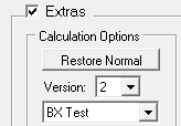
To further explore the impact of the not-so-hot "fundamental assumption", we built an option into TView to use that approach instead of TView's normal methods.  On a plansheet's "Settings" tab, check the "Extras" box, and set the first pop-up to "BX Test", like this:

 

 

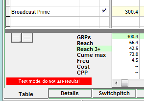
The main Table view will warn you that this setting is in effect, and that results will be prepared using the "fundamental assumption" as described by BrandX:

 

 

 

A Personal View of Respondents

 

With the wonders of real respondent data, we are able to predict schedule exposure for each individual in the panel. Since every person has a different viewing pattern, the best way to do this is to continue to treat them as individuals, even if several people have the overall same amount of viewing.